Visual tour of curvature matrices

This tutorial visualizes different curvature matrices for a model with sufficiently small parameter space.

First, the imports.

from typing import Callable, Tuple

import matplotlib.pyplot as plt
import numpy
import torch
from matplotlib.axes import Axes
from matplotlib.figure import Figure
from torch import nn

from curvlinops import EFLinearOperator, GGNLinearOperator, HessianLinearOperator

# make deterministic
torch.manual_seed(0)
numpy.random.seed(0)

DEVICE = torch.device("cuda" if torch.cuda.is_available() else "cpu")

Setup

We will create a synthetic classification task, a small CNN, and use cross-entropy error as loss function.

num_data = 50
batch_size = 20
in_channels = 3
in_features_shape = (in_channels, 10, 10)
num_classes = 5

# dataset
dataset = torch.utils.data.TensorDataset(
    torch.rand(num_data, *in_features_shape),  # X
    torch.randint(size=(num_data,), low=0, high=num_classes),  # y
)
dataloader = torch.utils.data.DataLoader(dataset, batch_size=batch_size)

# model
model = nn.Sequential(
    nn.Conv2d(in_channels, 4, 3, padding=1),
    nn.ReLU(),
    nn.Conv2d(4, 4, 5, padding=2, stride=2),
    nn.Sigmoid(),
    nn.Conv2d(4, 1, 3, padding=1),
    nn.Flatten(),
    nn.Linear(25, num_classes),
).to(DEVICE)

params = [p for p in model.parameters() if p.requires_grad]
num_params = sum(p.numel() for p in params)
num_params_layer = [
    sum(p.numel() for p in child.parameters()) for child in model.children()
]

loss_function = nn.CrossEntropyLoss(reduction="mean").to(DEVICE)

print(f"Total parameters: {num_params}")
print(f"Layer parameters: {num_params_layer}")

Total parameters: 683
Layer parameters: [112, 0, 404, 0, 37, 0, 130]

Computation

We can now set up linear operators for the curvature matrices we want to visualize, and compute them by multiplying the linear operator onto the identity matrix.

First, create the linear operators:

Hessian_linop = HessianLinearOperator(model, loss_function, params, dataloader)
GGN_linop = GGNLinearOperator(model, loss_function, params, dataloader)
EF_linop = EFLinearOperator(model, loss_function, params, dataloader)

Then, compute the matrices

identity = numpy.eye(num_params).astype(Hessian_linop.dtype)

Hessian_mat = Hessian_linop @ identity
GGN_mat = GGN_linop @ identity
EF_mat = EF_linop @ identity

Visualization

We will show the matrix entries on a shared domain for better comparability.

matrices = [Hessian_mat, GGN_mat, EF_mat]
titles = ["Hessian", "GGN", "Empirical Fisher"]

rows, columns = 1, 3
img_width = 7


def plot(
    transform: Callable[[numpy.ndarray], numpy.ndarray], transform_title: str = None
) -> Tuple[Figure, Axes]:
    """Visualize transformed curvature matrices using a shared domain.

    Args:
        transform: A transformation that will be applied to the matrices. Must
            accept a matrix and return a matrix of the same shape.
        transform_title: An optional string describing the transformation.
            Default: `None` (empty).

    Returns:
        Figure and axes of the created subplot.
    """
    min_value = min(transform(mat).min() for mat in matrices)
    max_value = max(transform(mat).max() for mat in matrices)

    fig, axes = plt.subplots(
        nrows=rows, ncols=columns, figsize=(columns * img_width, rows * img_width)
    )

    for idx, (ax, mat, title) in enumerate(zip(axes.flat, matrices, titles)):
        ax.set_title(title)
        img = ax.imshow(transform(mat), vmin=min_value, vmax=max_value)

        # layer structure
        for pos in numpy.cumsum(num_params_layer):
            if pos not in [0, num_params]:
                style = {"color": "w", "lw": 0.5, "ls": "--"}
                ax.axhline(y=pos - 1, xmin=0, xmax=num_params - 1, **style)
                ax.axvline(x=pos - 1, ymin=0, ymax=num_params - 1, **style)

        # colorbar
        last = idx == len(matrices) - 1
        if last:
            fig.colorbar(
                img, ax=axes.ravel().tolist(), label=transform_title, shrink=0.8
            )

    return fig, axes

We will show their logarithmic absolute value:

def logabs(mat, epsilon=1e-5):
    return numpy.log10(numpy.abs(mat) + epsilon)


plot(logabs, transform_title="Logarithmic absolute entries")

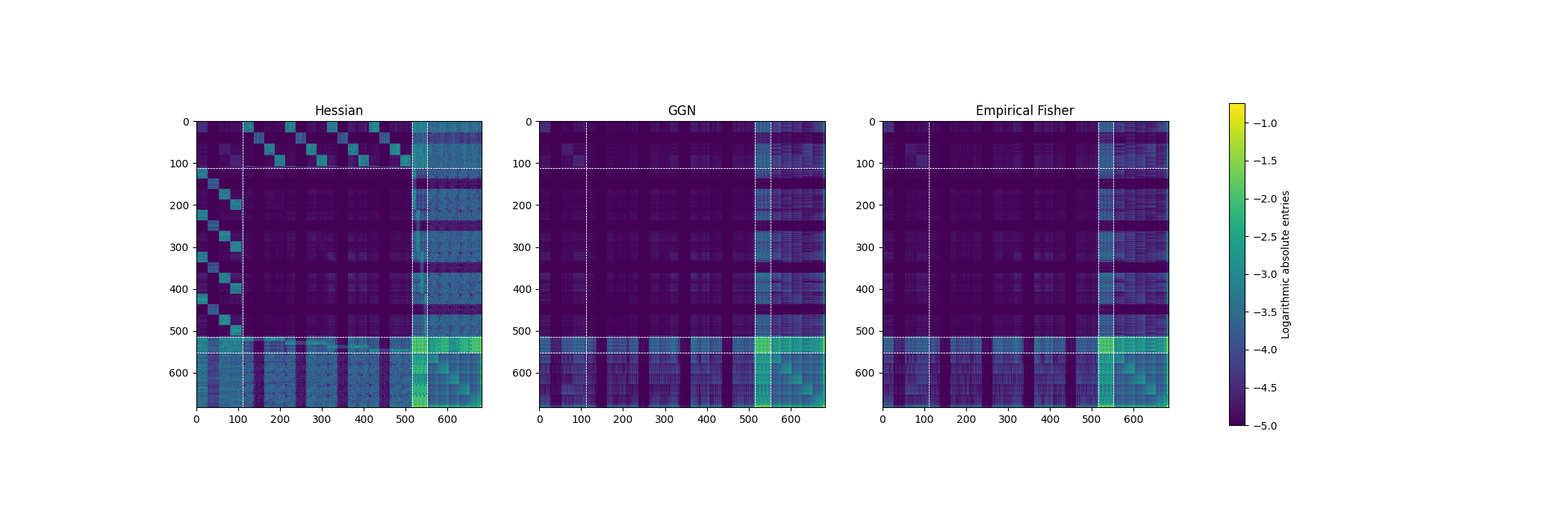
(<Figure size 2100x700 with 4 Axes>, array([<Axes: title={'center': 'Hessian'}>,
       <Axes: title={'center': 'GGN'}>,
       <Axes: title={'center': 'Empirical Fisher'}>], dtype=object))

That’s because it is hard to recognize structure in the unaltered entries:

def unchanged(mat):
    return mat


plot(unchanged, transform_title="Unaltered matrix entries")

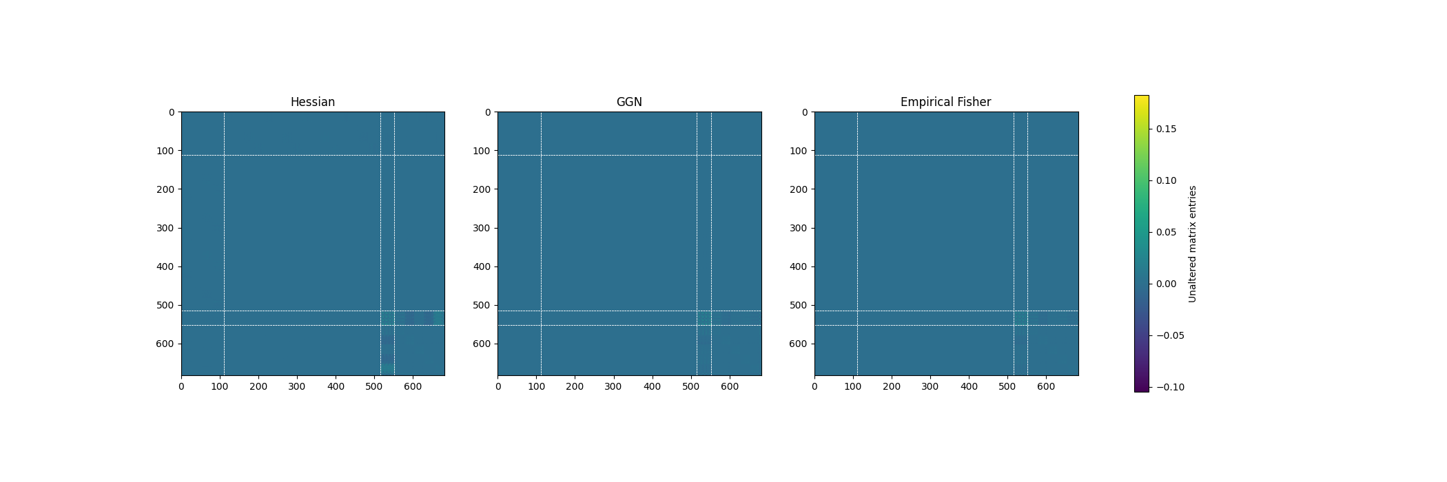
(<Figure size 2100x700 with 4 Axes>, array([<Axes: title={'center': 'Hessian'}>,
       <Axes: title={'center': 'GGN'}>,
       <Axes: title={'center': 'Empirical Fisher'}>], dtype=object))

That’s all for now.

plt.close("all")