Spectral density estimation (verification)

In this example we will use the spectral density estimation techniques of Papyan, 2020 to reproduce the plots for synthetic spectra shown in Figure 15 of the paper.

Here are the imports:

import matplotlib.pyplot as plt
from numpy import e, exp, linspace, log, logspace, matmul, ndarray, zeros
from numpy.linalg import eigh
from numpy.random import pareto, randn, seed
from scipy.sparse.linalg import aslinearoperator, eigsh

from curvlinops.outer import OuterProductLinearOperator
from curvlinops.papyan2020traces.spectrum import (
    LanczosApproximateLogSpectrumCached,
    LanczosApproximateSpectrumCached,
    lanczos_approximate_log_spectrum,
    lanczos_approximate_spectrum,
)

seed(0)

Approximating a spectrum

The first subplot (Figure 15a) uses a synthetic matrix \(\mathbf{Y} = \mathbf{X} + \mathbf{Z} \mathbf{Z}^\top \in \mathbb{R}^{2000 \times 2000}\) where \(\mathbf{X}_{1,1} = 5\), \(\mathbf{X}_{2,2} = 4\), \(\mathbf{X}_{3,3} = 3\) and zero elsewhere, and the elements of \(\mathbf{Z} \in \mathbb{R}^{2000 \times 2000}\) are standard normally distributed.

Here is the function to draw a sample for \(\mathbf{Y}\):

def create_matrix(dim: int = 2000) -> ndarray:
    """Draw a matrix from the matrix distribution used in papyan2020traces, Figure 15a.

    Args:
        dim: Matrix dimension.

    Returns:
        A sample from the matrix distribution.k
    """
    X = zeros((dim, dim))
    X[0, 0] = 5
    X[1, 1] = 4
    X[2, 2] = 3

    Z = randn(dim, dim)

    return X + 1 / dim * matmul(Z, Z.transpose())


Y = create_matrix()

This matrix is still reasonably small to compute its eigen-decomposition

print("Computing the full spectrum")
Y_evals, _ = eigh(Y)

Computing the full spectrum

For an approximation of the eigenvalue spectrum we just need a LinearOperator of Y:

Y_linop = aslinearoperator(Y)

Without rank deflation

We can now approximate the approximate spectrum using lanczos_approximate_spectrum and using the same hyperparameters as specified by the paper:

# spectral density hyperparameters
num_points = 1024
ncv = 128
num_repeats = 10
kappa = 3
margin = 0.05

For convenience, we feed the eigenvalues at the spectrum’s edges as boundaries, so they don’t get recomputed:

boundaries = (Y_evals.min(), Y_evals.max())

Let’s compute the approximate spectrum

print("Approximating density")
grid, density = lanczos_approximate_spectrum(
    Y_linop,
    ncv,
    num_points=num_points,
    num_repeats=num_repeats,
    kappa=kappa,
    boundaries=boundaries,
    margin=margin,
)

Approximating density

and plot it with a histogram (same number of bins as in the paper) of the exact density:

plt.figure()
plt.xlabel("Eigenvalue")
plt.ylabel("Spectral density")

left, right = grid[0], grid[-1]
num_bins = 100
bins = linspace(left, right, num_bins, endpoint=True)
plt.hist(Y_evals, bins=bins, log=True, density=True, label="Exact")

plt.plot(grid, density, label="Approximate")
plt.legend()

# same ylimits as in the paper
plt.ylim(bottom=1e-5, top=1e1)

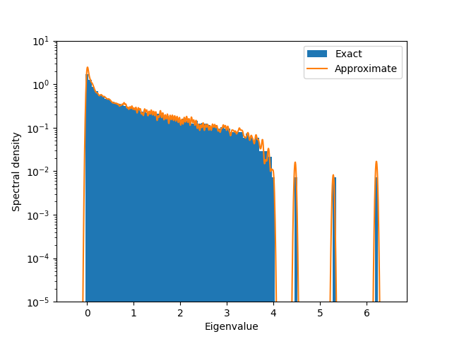
(1e-05, 10.0)

For multiple hyperparameters

You may have noticed that there are multiple hyperparameters in the spectra estimation method. For instance, the kappa parameter, which determines the width of the superimposed Gaussian bumps. In practice, this parameter requires tuning. But trying out another value with the above approach needs to re-evaluate the Lanczos iterations. This quickly becomes expensive, especially for larger matrices.

As a solution, there exists a class LanczosApproximateSpectrumCached that computes and caches Lanczos iterations as we need them. This allows to quickly try out multiple hyperparameters.

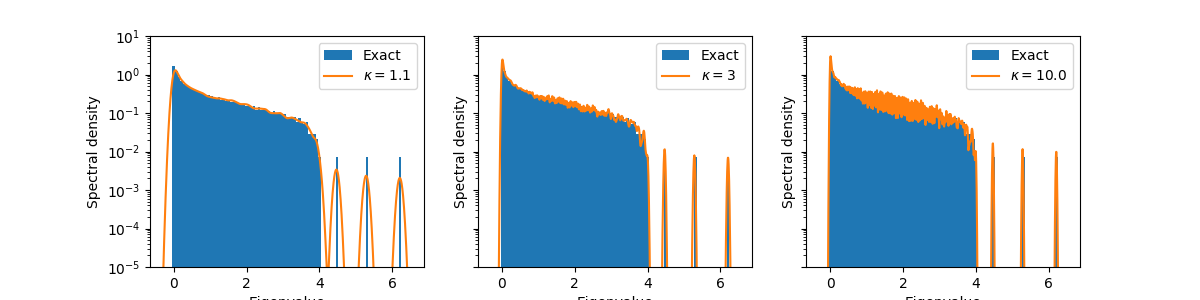
Let’s try out different values for kappa:

kappas = [1.1, 3, 10.0]
fig, ax = plt.subplots(ncols=len(kappas), figsize=(12, 3), sharex=True, sharey=True)

cache = LanczosApproximateSpectrumCached(Y_linop, ncv, boundaries)

for idx, kappa in enumerate(kappas):
    grid, density = cache.approximate_spectrum(
        num_repeats=num_repeats, num_points=num_points, kappa=kappa, margin=margin
    )

    ax[idx].hist(Y_evals, bins=bins, log=True, density=True, label="Exact")
    ax[idx].plot(grid, density, label=rf"$\kappa = {kappa}$")
    ax[idx].legend()

    ax[idx].set_xlabel("Eigenvalue")
    ax[idx].set_ylabel("Spectral density")
    ax[idx].set_ylim(bottom=1e-5, top=1e1)

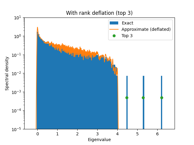
Wit rank deflation

As you can see in the above plot, the spectrum consists of a bulk and three outliers. We can project out the three (or in general k) outliers to increase the approximation of the bulk. This technique is called rank deflation.

k = 3
print(f"Computing top-{k} eigenvalues of normalized operator")
Y_top_evals, Y_top_evecs = eigsh(Y_linop, k=k, which="LA")

Y_top_linop = OuterProductLinearOperator(Y_top_evals, Y_top_evecs)

Y_deflated_linop = Y_linop - Y_top_linop

Computing top-3 eigenvalues of normalized operator

The procedure to estimate the deflated operator’s spectral density is analogous:

print(f"Approximating density with eliminated top-{k} eigenspace")
grid_no_top, density_no_top = lanczos_approximate_spectrum(
    Y_deflated_linop,
    ncv,
    num_points=num_points,
    num_repeats=num_repeats,
    kappa=kappa,
    boundaries=boundaries,
    margin=0.05,
)

Approximating density with eliminated top-3 eigenspace

Here is the visualization, with outliers marked separately:

plt.figure()
plt.title(f"With rank deflation (top {k})")
plt.xlabel("Eigenvalue")
plt.ylabel("Spectral density")

plt.hist(Y_evals, bins=bins, log=True, density=True, label="Exact")
plt.plot(grid_no_top, density_no_top, label="Approximate (deflated)")

plt.plot(
    Y_top_evals,
    len(Y_top_evals) * [1 / Y_linop.shape[0]],
    linestyle="",
    marker="o",
    label=f"Top {k}",
)

# same ylimits as in the paper
plt.ylim(bottom=1e-5, top=1e1)
plt.legend()

<matplotlib.legend.Legend object at 0x7a294ba566d0>

Approximating a log-spectrum

The second subplot (Figure 15b) uses a synthetic matrix \(\mathbf{Y} = \frac{1}{1000} \mathbf{Z} \mathbf{Z}^\top \in \mathbb{R}^{500 \times 500}\) where the elements of \(\mathbf{Z} \in \mathbb{R}^{500 \times 1000}\) are following an i.i.d. Pareto distribution with parameter \(\alpha = 1\).

Here is the function to draw a sample for \(\mathbf{Y}\):

seed(0)


def create_matrix_log_spectrum(dim: int = 500) -> ndarray:
    """Draw a matrix from the matrix distribution used in papyan2020traces, Figure 15b.

    Args:
        dim: Matrix dimension.

    Returns:
        A sample from the matrix distribution.
    """
    Z = pareto(a=1, size=(dim, 2 * dim))

    return 1 / (2 * dim) * Z @ Z.transpose()


Y = create_matrix_log_spectrum()

As we will see below, the spectrum of such a matrix spans a large range. It is therefore interesting to estimate the spectral density not on a linear (\(p(\lambda)\)), but on a logarithmic scale (\(p(\log|\lambda|)\)).

We will therefore consider estimating the spectral density of \(\log(|\mathbf{A}| + \epsilon \mathbf{I})\) where the absolute value refers to replacing an eigenvalue of \(\mathbf{Y}\) by its magnitude (likewise for the \(\log\) operation). \(\epsilon\) is a small shift to guarantee the logarithm exists.

epsilon = 1e-5

Let’s start by computing the exact spectrum and generating a linear operator:

print("Computing the full log-spectrum")
Y_evals, _ = eigh(Y)

Y_linop = aslinearoperator(Y)

Computing the full log-spectrum

We can now approximate the approximate log-spectrum using lanczos_approximate_log_spectrum and using the same hyperparameters as specified by the paper:

# spectral density hyperparameters
num_points = 1024
margin = 0.05
ncv = 256
num_repeats = 10
kappa = 1.04  # not specified in the paper → hand-tuned

For convenience, we feed the eigenvalue magnitudes at the spectrum’s edges as boundaries, so they don’t get recomputed:

Y_abs_evals = abs(Y_evals)
boundaries = (Y_abs_evals.min(), Y_abs_evals.max())

print("Approximating log-spectrum")
grid, density = lanczos_approximate_log_spectrum(
    Y_linop,
    ncv,
    num_points=num_points,
    num_repeats=num_repeats,
    kappa=kappa,
    boundaries=boundaries,
    margin=margin,
    epsilon=epsilon,
)

Approximating log-spectrum

Now we can visualize the results:

plt.figure()
plt.xlabel("Eigenvalue")
plt.ylabel("Spectral density")

Y_log_abs_evals = log(abs(Y_evals) + epsilon)

xlimits_no_margin = (Y_log_abs_evals.min(), Y_log_abs_evals.max())
width_no_margins = xlimits_no_margin[1] - xlimits_no_margin[0]
xlimits = [
    xlimits_no_margin[0] - margin * width_no_margins,
    xlimits_no_margin[1] + margin * width_no_margins,
]

plt.semilogx()
num_bins = 100
bins = logspace(*xlimits, num=num_bins, endpoint=True, base=e)
plt.hist(exp(Y_log_abs_evals), bins=bins, log=True, density=True, label="Exact")

plt.plot(grid, density, label="Approximate")

# use same ylimits as in the paper
plt.ylim(bottom=1e-14, top=1e-2)
plt.legend()

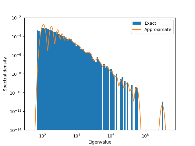
<matplotlib.legend.Legend object at 0x7a2950b1eca0>

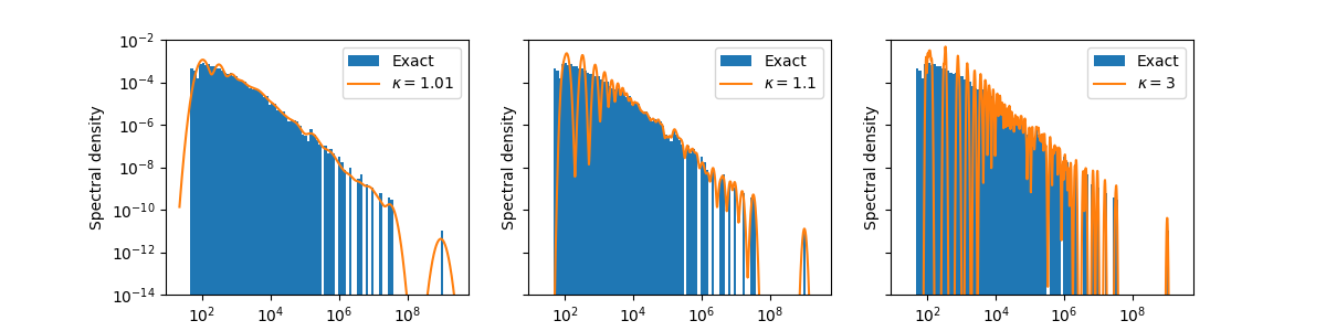
For multiple hyperparameters

To efficiently produce such plots for multiple hyperparameters, there exists a class LanczosApproximateLogSpectrumCached that computes and caches Lanczos iterations as we need them.

Let’s try out different values for kappa:

plt.close()

kappas = [1.01, 1.1, 3]
fig, ax = plt.subplots(ncols=len(kappas), figsize=(12, 3), sharex=True, sharey=True)

cache = LanczosApproximateLogSpectrumCached(Y_linop, ncv, boundaries)

for idx, kappa in enumerate(kappas):
    grid, density = cache.approximate_log_spectrum(
        num_repeats=num_repeats,
        num_points=num_points,
        kappa=kappa,
        margin=margin,
        epsilon=epsilon,
    )

    ax[idx].hist(exp(Y_log_abs_evals), bins=bins, log=True, density=True, label="Exact")
    ax[idx].loglog(grid, density, label=rf"$\kappa = {kappa}$")
    ax[idx].legend()

    ax[idx].set_xlabel("Eigenvalue")
    ax[idx].set_ylabel("Spectral density")
    ax[idx].set_ylim(bottom=1e-14, top=1e-2)