Inverses (natural gradient)

This example demonstrates how to work with inverses of linear operators.

curvlinops offers multiple ways to compute the inverse of a linear operator: conjugate gradient (CG) and Neumann inversion. We will demonstrate CG inversion first and conclude with a comparison to Neumann inversion.

Concretely, we will compute the natural gradient \(\mathbf{\tilde{g}} = \mathbf{F}^{-1} \mathbf{g}\), defined by the inverse Fisher information matrix \(\mathbf{F}^{-1}\) and the gradient \(\mathbf{g}\). We can use the GGN, as it corresponds to the Fisher for common loss functions like square and cross-entropy loss.

Note

The GGN is positive semi-definite, i.e. not full-rank. But we need a full-rank matrix to form the inverse. This is why we will add a damping term \(\delta \mathbf{I}\) before inverting.

As always, let’s first import the required functionality.

import matplotlib.pyplot as plt
import numpy
import torch
from scipy import sparse
from scipy.sparse.linalg import aslinearoperator, eigsh
from torch import nn

from curvlinops import (
    CGInverseLinearOperator,
    GGNLinearOperator,
    NeumannInverseLinearOperator,
)
from curvlinops.examples.functorch import functorch_ggn, functorch_gradient
from curvlinops.examples.utils import report_nonclose

# make deterministic
torch.manual_seed(0)
numpy.random.seed(0)

Setup

We will use synthetic data, consisting of two mini-batches, a small MLP, and mean-squared error as loss function.

N = 20
D_in = 7
D_hidden = 5
D_out = 3

DEVICE = torch.device("cuda" if torch.cuda.is_available() else "cpu")

X1, y1 = torch.rand(N, D_in).to(DEVICE), torch.rand(N, D_out).to(DEVICE)
X2, y2 = torch.rand(N, D_in).to(DEVICE), torch.rand(N, D_out).to(DEVICE)

model = nn.Sequential(
    nn.Linear(D_in, D_hidden),
    nn.ReLU(),
    nn.Linear(D_hidden, D_hidden),
    nn.Sigmoid(),
    nn.Linear(D_hidden, D_out),
).to(DEVICE)
params = [p for p in model.parameters() if p.requires_grad]

loss_function = nn.MSELoss(reduction="mean").to(DEVICE)


# %
#
# Next, let's compute the ingredients for the natural gradient.
#
# Inverse GGN/Fisher
# ------------------
#
# First,  we set up a linear operator for the damped GGN/Fisher

data = [(X1, y1), (X2, y2)]
GGN = GGNLinearOperator(model, loss_function, params, data)

delta = 1e-2
damping = aslinearoperator(delta * sparse.eye(GGN.shape[0]))

damped_GGN = GGN + damping

and the linear operator of its inverse:

inverse_damped_GGN = CGInverseLinearOperator(damped_GGN)

Gradient

We can obtain the gradient via a convenience function of GGNLinearOperator:

gradient, _ = GGN.gradient_and_loss()
# convert to numpy (vector) format
gradient = nn.utils.parameters_to_vector(gradient).cpu().detach()

Natural gradient

Now we have all components together to compute the natural gradient with a simple matrix-vector product:

natural_gradient = inverse_damped_GGN @ gradient

/home/docs/checkouts/readthedocs.org/user_builds/curvlinops/envs/1.2.0/lib/python3.8/site-packages/curvlinops/_base.py:259: UserWarning: Input vector is float64, while linear operator is float32. Converting to float32.
  warn(

As a first sanity check, let’s compare if the natural gradient satisfies \(\mathbf{F} \mathbf{\tilde{g}} = \mathbf{g}\)

approx_gradient = damped_GGN @ natural_gradient

print("Comparing gradient with Fisher @ natural gradient.")
report_nonclose(approx_gradient, gradient, rtol=1e-4, atol=1e-5)

Comparing gradient with Fisher @ natural gradient.
Compared arrays match.

Verifying results

To check if the code works, let’s compute the GGN with functorch, using a utility function of curvlinops.examples; then damp it, invert it, and multiply it onto the gradient.

GGN_mat_functorch = (
    functorch_ggn(model, loss_function, params, data).detach().cpu().numpy()
)

then damp it and invert it.

damping_mat = delta * numpy.eye(GGN_mat_functorch.shape[0])
damped_GGN_mat = GGN_mat_functorch + damping_mat
inv_damped_GGN_mat = numpy.linalg.inv(damped_GGN_mat)

Next, let’s compute the gradient with functorch, using a utility function from curvlinops.examples:

gradient_functorch = functorch_gradient(model, loss_function, params, data)
# convert to numpy (vector) format
gradient_functorch = (
    nn.utils.parameters_to_vector(gradient_functorch).detach().cpu().numpy()
)

print("Comparing gradient with functorch's gradient.")
report_nonclose(gradient, gradient_functorch)

Comparing gradient with functorch's gradient.
Compared arrays match.

We can now compute the natural gradient from the :code:`functorch `quantities. This should yield approximately the same result:

natural_gradient_functorch = inv_damped_GGN_mat @ gradient_functorch

print("Comparing natural gradient with functorch's natural gradient.")
rtol, atol = 5e-3, 1e-5
report_nonclose(natural_gradient, natural_gradient_functorch, rtol=rtol, atol=atol)

Comparing natural gradient with functorch's natural gradient.
Compared arrays match.

You might have noticed the rather small tolerances required to achieve approximate equality. We can use stricter convergence hyperparameters for CG to achieve a more accurate inversion

inverse_damped_GGN.set_cg_hyperparameters(tol=1e-7)  # default is 1e-5
natural_gradient_more_accurate = inverse_damped_GGN @ gradient

smaller_rtol, smaller_atol = rtol / 10, atol / 10
print("Comparing more accurate natural gradient with functorch's natural gradient.")
report_nonclose(
    natural_gradient_more_accurate,
    natural_gradient_functorch,
    rtol=smaller_rtol,
    atol=smaller_atol,
)

Comparing more accurate natural gradient with functorch's natural gradient.
Compared arrays match.

whereas the less accurate inversion does not pass this check:

print(
    "Comparing natural gradient with functorch's natural gradient (smaller tolerances)."
)
try:
    report_nonclose(
        natural_gradient,
        natural_gradient_functorch,
        rtol=smaller_rtol,
        atol=smaller_atol,
    )
    raise RuntimeError("This comparison should not pass")
except ValueError as e:
    print(e)

Comparing natural gradient with functorch's natural gradient (smaller tolerances).
0.001005700484743552 ≠ 0.0010132172898633662 (ratio 0.99258)
-0.00014257251718040464 ≠ -0.00013771530795653186 (ratio 1.03527)
-0.018138318591713283 ≠ -0.018126217200963746 (ratio 1.00067)
-0.0007731041536374922 ≠ -0.000783620053370071 (ratio 0.98658)
-0.006884070281747075 ≠ -0.006893014821781007 (ratio 0.99870)
-0.0034347233329645394 ≠ -0.00344548142884199 (ratio 0.99688)
-0.01250206732905876 ≠ -0.012493652614168516 (ratio 1.00067)
0.01160294660905081 ≠ 0.011610329754090709 (ratio 0.99936)
0.0010863092835098303 ≠ 0.001093295386912052 (ratio 0.99361)
-0.010272672285824147 ≠ -0.01028052241702504 (ratio 0.99924)
-0.0002681519717021947 ≠ -0.00026666751640896935 (ratio 1.00557)
Max: 0.17760, 0.17760
Min: -0.29772, -0.29772
Compared arrays don't match.

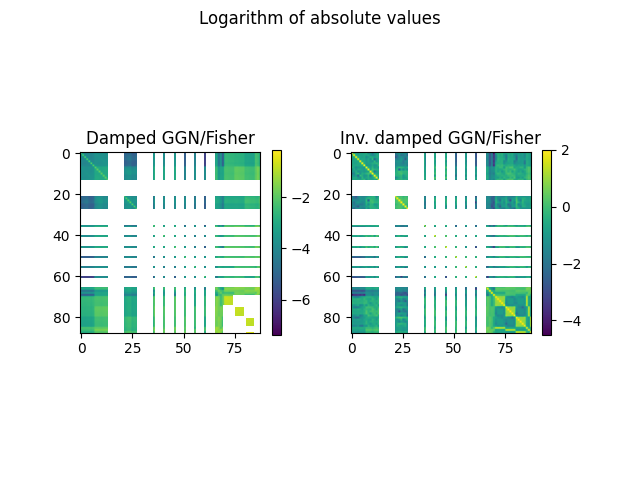
Visual comparison

Finally, let’s visualize the damped Fisher/GGN and its inverse. For improved visibility, we take the logarithm of the absolute value of each element (blank pixels correspond to zeros).

fig, ax = plt.subplots(ncols=2)
plt.suptitle("Logarithm of absolute values")

ax[0].set_title("Damped GGN/Fisher")
image = ax[0].imshow(numpy.log10(numpy.abs(damped_GGN_mat)))
plt.colorbar(image, ax=ax[0], shrink=0.5)

ax[1].set_title("Inv. damped GGN/Fisher")
image = ax[1].imshow(numpy.log10(numpy.abs(inv_damped_GGN_mat)))
plt.colorbar(image, ax=ax[1], shrink=0.5)

/home/docs/checkouts/readthedocs.org/user_builds/curvlinops/checkouts/1.2.0/docs/examples/basic_usage/example_inverses.py:223: RuntimeWarning: divide by zero encountered in log10
  image = ax[0].imshow(numpy.log10(numpy.abs(damped_GGN_mat)))
/home/docs/checkouts/readthedocs.org/user_builds/curvlinops/checkouts/1.2.0/docs/examples/basic_usage/example_inverses.py:227: RuntimeWarning: divide by zero encountered in log10
  image = ax[1].imshow(numpy.log10(numpy.abs(inv_damped_GGN_mat)))

<matplotlib.colorbar.Colorbar object at 0x7a294e74d5b0>

Neumann inverse (CG alternative)

So far, we used CG to solve the linear system \(\mathbf{F} \mathbf{\tilde{g}} = \mathbf{g}\) for the natural gradient \(\mathbf{\tilde{g}}\) (i.e. the result of the inverse Fisher-gradient product). Alternatively, we can use the truncated Neumann series to approximate the inverse, using NeumannLinearOperator.

Note

The Neumann series does not always converge. But we can use a re-scaling trick to make it converge if we know the matrix is PSD and are given its largest eigenvalue. More information can be found in the docstring.

To make the Neumann series converge, we need to know the largest eigenvalue of the matrix to be inverted:

max_eigval = eigsh(damped_GGN, k=1, which="LM", return_eigenvectors=False)[0]
# eigenvalues (scale * damped_GGN_mat) are in [0; 2)
scale = 1.0 if max_eigval < 2.0 else 1.99 / max_eigval

Let’s compute the inverse approximation for different truncation numbers:

num_terms = [10]
neumann_inverses = []

for n in num_terms:
    inv = NeumannInverseLinearOperator(damped_GGN, scale=scale, num_terms=n)
    neumann_inverses.append(inv @ numpy.eye(inv.shape[1]))

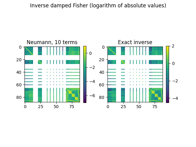
Here are their visualizations:

fig, axes = plt.subplots(ncols=len(num_terms) + 1)
plt.suptitle("Inverse damped Fisher (logarithm of absolute values)")

for i, (n, inv) in enumerate(zip(num_terms, neumann_inverses)):
    ax = axes.flat[i]
    ax.set_title(f"Neumann, {n} terms")
    image = ax.imshow(numpy.log10(numpy.abs(inv)))
    plt.colorbar(image, ax=ax, shrink=0.5)

ax = axes.flat[-1]
ax.set_title("Exact inverse")
image = ax.imshow(numpy.log10(numpy.abs(inv_damped_GGN_mat)))
plt.colorbar(image, ax=ax, shrink=0.5)

/home/docs/checkouts/readthedocs.org/user_builds/curvlinops/checkouts/1.2.0/docs/examples/basic_usage/example_inverses.py:274: RuntimeWarning: divide by zero encountered in log10
  image = ax.imshow(numpy.log10(numpy.abs(inv)))
/home/docs/checkouts/readthedocs.org/user_builds/curvlinops/checkouts/1.2.0/docs/examples/basic_usage/example_inverses.py:279: RuntimeWarning: divide by zero encountered in log10
  image = ax.imshow(numpy.log10(numpy.abs(inv_damped_GGN_mat)))

<matplotlib.colorbar.Colorbar object at 0x7a2950af0ca0>

The Neumann inversion is usually more inaccurate than CG inversion. But it might sometimes be preferred if only a rough approximation of the inverse matrix product is needed.