Matrix-vector products

This tutorial contains a basic demonstration how to set up LinearOperators for the Hessian and the GGN and how to multiply them to a vector.

First, the imports.

import matplotlib.pyplot as plt
import numpy
import torch
from torch import nn

from curvlinops import GGNLinearOperator, HessianLinearOperator
from curvlinops.examples.functorch import functorch_ggn, functorch_hessian
from curvlinops.examples.utils import report_nonclose

# make deterministic
torch.manual_seed(0)
numpy.random.seed(0)

Setup

Let’s create some toy data, a small MLP, and use mean-squared error as loss function.

N = 4
D_in = 7
D_hidden = 5
D_out = 3

DEVICE = torch.device("cuda" if torch.cuda.is_available() else "cpu")

X = torch.rand(N, D_in).to(DEVICE)
y = torch.rand(N, D_out).to(DEVICE)

model = nn.Sequential(
    nn.Linear(D_in, D_hidden),
    nn.ReLU(),
    nn.Linear(D_hidden, D_hidden),
    nn.Sigmoid(),
    nn.Linear(D_hidden, D_out),
).to(DEVICE)
params = [p for p in model.parameters() if p.requires_grad]

loss_function = nn.MSELoss(reduction="mean").to(DEVICE)

Hessian-vector products

Setting up a linear operator for the Hessian is straightforward.

data = [(X, y)]
H = HessianLinearOperator(model, loss_function, params, data)

We can now multiply by the Hessian. This operation will be carried out in PyTorch under the hood, but the operator is compatible with scipy, so we can just pass a numpy vector to the matrix-multiplication.

D = H.shape[0]
v = numpy.random.rand(D)

Hv = H @ v

/home/docs/checkouts/readthedocs.org/user_builds/curvlinops/envs/1.2.0/lib/python3.8/site-packages/curvlinops/_base.py:259: UserWarning: Input vector is float64, while linear operator is float32. Converting to float32.
  warn(

To verify the result, we compute the Hessian using functorch, using a utility function from curvlinops.examples:

H_mat = functorch_hessian(model, loss_function, params, data).detach().cpu().numpy()

Let’s check that the multiplication onto v leads to the same result:

Hv_functorch = H_mat @ v

print("Comparing Hessian-vector product with functorch's Hessian-vector product.")
report_nonclose(Hv, Hv_functorch)

Comparing Hessian-vector product with functorch's Hessian-vector product.
Compared arrays match.

Hessian-matrix products

We can also compute the Hessian’s matrix representation with the linear operator, simply by multiplying it onto the identity matrix. (Of course, this only works if the Hessian is small enough.)

H_mat_from_linop = H @ numpy.eye(D)

This should yield the same matrix as with functorch.

print("Comparing Hessian with functorch's Hessian.")
report_nonclose(H_mat, H_mat_from_linop)

Comparing Hessian with functorch's Hessian.
Compared arrays match.

Last, here’s a visualization of the Hessian.

plt.figure()
plt.title("Hessian")
plt.imshow(H_mat)
plt.colorbar()

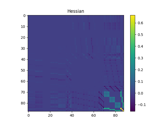
<matplotlib.colorbar.Colorbar object at 0x7a2952c667c0>

GGN-vector products

Setting up a linear operator for the Fisher/GGN is identical to the Hessian.

GGN = GGNLinearOperator(model, loss_function, params, data)

Let’s compute a GGN-vector product.

D = H.shape[0]
v = numpy.random.rand(D)

GGNv = GGN @ v

To verify the result, we will use functorch to compute the GGN. For that, we use that the GGN corresponds to the Hessian if we replace the neural network by its linearization. This is implemented in a utility function of curvlinops.examples:

GGN_mat = functorch_ggn(model, loss_function, params, data).detach().cpu().numpy()

GGNv_functorch = GGN_mat @ v

print("Comparing GGN-vector product with functorch's GGN-vector product.")
report_nonclose(GGNv, GGNv_functorch)

Comparing GGN-vector product with functorch's GGN-vector product.
Compared arrays match.

GGN-matrix products

We can also compute the GGN matrix representation with the linear operator, simply by multiplying it onto the identity matrix. (Of course, this only works if the GGN is small enough.)

GGN_mat_from_linop = GGN @ numpy.eye(D)

This should yield the same matrix as with functorch.

print("Comparing GGN with functorch's GGN.")
report_nonclose(GGN_mat, GGN_mat_from_linop)

Comparing GGN with functorch's GGN.
Compared arrays match.

Last, here’s a visualization of the GGN.

plt.figure()
plt.title("GGN")
plt.imshow(GGN_mat)
plt.colorbar()

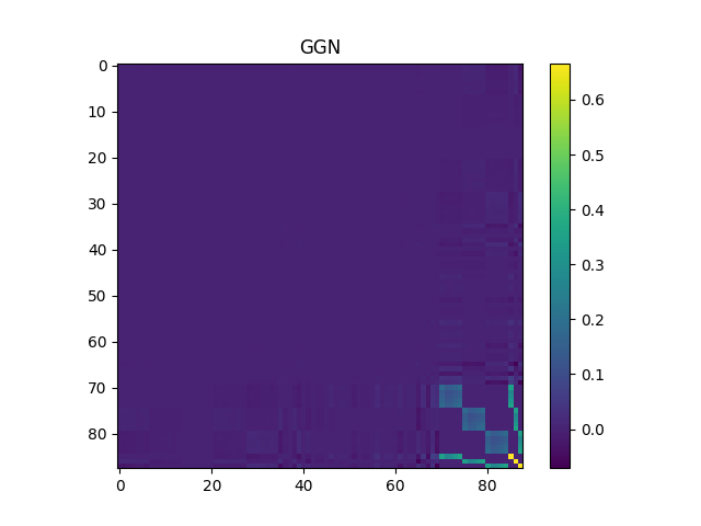
<matplotlib.colorbar.Colorbar object at 0x7a2950b16df0>

Visual comparison: Hessian and GGN

To conclude, let’s plot both the Hessian and GGN using the same limits

min_value = min(GGN_mat.min(), H_mat.min())
max_value = max(GGN_mat.max(), H_mat.max())

fig, ax = plt.subplots(ncols=2)
ax[0].set_title("Hessian")
ax[0].imshow(H_mat, vmin=min_value, vmax=max_value)
ax[1].set_title("GGN")
ax[1].imshow(GGN_mat, vmin=min_value, vmax=max_value)

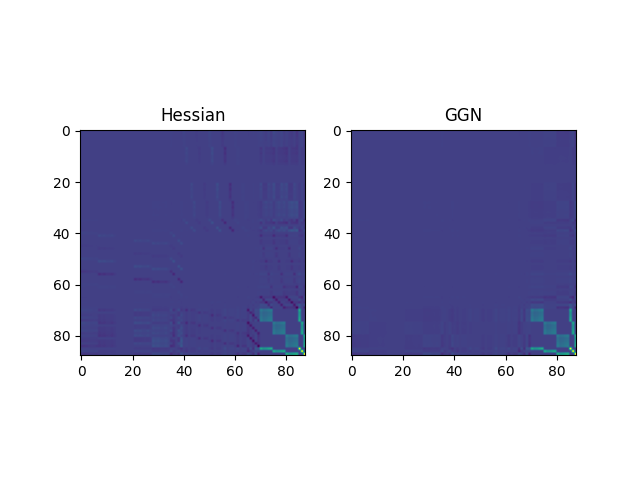
<matplotlib.image.AxesImage object at 0x7a2950ab1370>