Note
Go to the end to download the full example code.
Trace and diagonal estimation
In this example we will explore estimators for the trace and diagonal of a matrix.
curvlinops implements different methods, and we will reproduce the results
from their original papers, using toy matrices with a power law spectrum.
Here are the imports:
from os import getenv
from shutil import which

import matplotlib.pyplot as plt
from torch import (
    Tensor,
    arange,
    as_tensor,
    float64,
    int32,
    linspace,
    manual_seed,
    median,
    quantile,
    randn,
    stack,
)
from torch.linalg import qr
from tueplots import bundles

from curvlinops import hutchinson_diag, hutchinson_trace, hutchpp_trace, xdiag, xtrace
from curvlinops.examples import TensorLinearOperator

# We want to analyze smaller matrices on RTD to reduce build time
RTD = getenv("READTHEDOCS")
# Use LaTeX if available
USETEX = which("latex") is not None

PLOT_CONFIG = bundles.icml2024(column="full" if RTD else "half", usetex=USETEX, nrows=2)

# Dimension of the matrices whose traces we will estimate
DIM = 200 if RTD else 1000
# Number of repeats for the Hutchinson estimator to compute error bars
NUM_REPEATS = 50 if RTD else 200

manual_seed(0)  # make deterministic
<torch._C.Generator object at 0x71fa6dd06810>
Setup
We will use power law matrices whose eigenvalues are given by \(\lambda_i = i^{-c}\), where \(i\) is the index of the eigenvalue and \(c\) is a constant that determines the rate of decay of the eigenvalues. A higher value of \(c\) results in a faster decay of the eigenvalues.
Here is a function that creates such a matrix:
def create_power_law_matrix(dim: int = DIM, c: float = 1.0) -> Tensor:
    """Draw a matrix with a power law spectrum.

    Eigenvalues λ_i are given by λ_i = i^(-c), where i is the index of the eigenvalue
    and c is a constant that determines the rate of decay of the eigenvalues.
    A higher value of c results in a faster decay of the eigenvalues.

    Args:
        dim: Matrix dimension.
        c: Power law constant. Default is ``1.0``.

    Returns:
        A sample matrix with a power law spectrum.
    """
    # Create the diagonal matrix Λ with Λii = i^(-c)
    L = (arange(1, dim + 1, dtype=float64) ** (-c)).diag()

    # Generate a random Gaussian matrix and orthogonalize it to get Q
    Q, _ = qr(randn(dim, dim, dtype=float64))

    # Construct the matrix A = Q^T Λ Q
    return Q.T @ L @ Q
Trace estimation
Basics
To get started, let’s create a power law matrix and turn it into a linear operator:
For reference, let’s compute the exact trace:
exact_trace = Y_mat.trace()
print(f"Exact trace: {exact_trace:.3f}")
Exact trace: 5.878
The simplest method for trace estimation is Hutchinson’s method.
The idea is to estimate the trace from matrix-vector products with random vectors. To obtain better estimates, we can use more queries. It is common to repeat this process multiple times to get error estimates.
Let’s estimate the trace and see if the estimate is decent:
# matrix-vector queries for one trace estimate
num_matvecs = 5
# Generate estimates, repeat process multiple times so we have error bars.
estimates = stack([hutchinson_trace(Y, num_matvecs) for _ in range(NUM_REPEATS)])
# Calculate the median and quartiles (error bars) of the estimates
med = median(estimates)
quartile1 = quantile(estimates, 0.25)
quartile3 = quantile(estimates, 0.75)
# Print the exact trace and the statistical measures of the estimates
print(f"Exact trace: {exact_trace:.3f}")
print("Estimate:")
print(f"\t- Median: {med:.3f}")
print(f"\t- First quartile (25%): {quartile1:.3f}")
print(f"\t- Third quartile (75%): {quartile3:.3f}")
# Also print whether the true value lies between the quartiles
is_within_quartiles = quartile1 <= exact_trace <= quartile3
print(f"True value within interquartile range? {is_within_quartiles}")
assert is_within_quartiles
Exact trace: 5.878
Estimate:
- Median: 5.965
- First quartile (25%): 5.565
- Third quartile (75%): 6.445
True value within interquartile range? True
Good! The estimate lies within the error bars.
Comparison
In the following, we will look at Hutchinson’s method and two other algorithms: Hutch++ and XTrace. Hutch++ combines vanilla Hutchinson with variance reduction, by deterministically computing the trace in a sub-space, and using Hutchinson’s method in the remaining space. XTrace uses variance reduction from Hutch++, and the exchangeability principle (i.e. the estimate is identical when permuting the random test vectors). All methods are unbiased, but Hutch++ and XTrace require additional memory to store the basis in which the trace is computed exactly.
For matrices whose trace is dominated by a few large eigenvalues, i.e. have fast spectral decay, Hutch++ and XTrace can converge faster than vanilla Hutchinson. For matrices with slow spectral decay, the benefits of Hutch++ and XTrace become less pronounced.
Let’s reproduce these results empirically.
We will first consider a power law matrix with high decay rate \(c=2.0\):
Y_mat = create_power_law_matrix(c=2.0)
As before, we will repeat the trace estimation to obtain error bars for each method, and investigate how their accuracy evolves as we increase the number of matrix-vector products. We use the relative error, which is the absolute value of the difference between the estimated and exact trace, divided by the exact trace’s absolute value.
Here is a function that computes these relative trace errors for a given matrix:
NUM_MATVECS_HUTCH = linspace(1, 100, 50, dtype=int32).unique()
# Hutch++ requires matrix-vector products divisible by 3
NUM_MATVECS_HUTCHPP = (NUM_MATVECS_HUTCH + (3 - NUM_MATVECS_HUTCH % 3)).unique()
# XTrace requires matrix-vector products divisible by 2
NUM_MATVECS_XTRACE = (NUM_MATVECS_HUTCH + (2 - NUM_MATVECS_HUTCH % 2)).unique()
def compute_relative_trace_errors(Y_mat: Tensor) -> dict[str, dict[str, Tensor]]:
"""Compute the relative trace errors for Hutchinson's method, Hutch++, and XTrace.
Args:
Y_mat: Matrix to estimate the trace of.
Returns:
Dictionary with the relative trace errors.
"""
Y = TensorLinearOperator(Y_mat)
exact_trace = Y_mat.trace()
# compute median and quartiles for Hutchinson's method
estimators = {
"Hutchinson": hutchinson_trace,
"Hutch++": hutchpp_trace,
"XTrace": xtrace,
}
num_matvecs = [NUM_MATVECS_HUTCH, NUM_MATVECS_HUTCHPP, NUM_MATVECS_XTRACE]
results = {}
for (name, method), num_matvecs_method in zip(estimators.items(), num_matvecs):
med = []
quartile1 = []
quartile3 = []
for n in num_matvecs_method:
estimates = stack([method(Y, n) for _ in range(NUM_REPEATS)])
errors = (estimates - exact_trace).abs() / abs(exact_trace)
med.append(median(errors))
quartile1.append(quantile(errors, 0.25))
quartile3.append(quantile(errors, 0.75))
results[name] = {
"med": as_tensor(med),
"quartile1": as_tensor(quartile1),
"quartile3": as_tensor(quartile3),
"num_matvecs": num_matvecs_method,
}
return results
Let’s compute the relative trace errors and look at them:
results = compute_relative_trace_errors(Y_mat)
print("Relative errors:")
for method, data in results.items():
print(f"-\t{method}:")
num_matvecs = data["num_matvecs"]
med = data["med"]
quartile1 = data["quartile1"]
quartile3 = data["quartile3"]
# print the first 3 values
for i in range(3):
print(
f"\t\t- {num_matvecs[i]} matvecs: median {med[i]:.5f}"
+ f" (quartiles {quartile1[i]:.3f} - {quartile3[i]:.3f})"
)
Relative errors:
- Hutchinson:
- 1 matvecs: median 0.51136 (quartiles 0.254 - 0.789)
- 3 matvecs: median 0.38620 (quartiles 0.255 - 0.561)
- 5 matvecs: median 0.25942 (quartiles 0.145 - 0.430)
- Hutch++:
- 3 matvecs: median 0.20786 (quartiles 0.104 - 0.314)
- 6 matvecs: median 0.07095 (quartiles 0.030 - 0.120)
- 9 matvecs: median 0.04516 (quartiles 0.025 - 0.076)
- XTrace:
- 2 matvecs: median 0.44112 (quartiles 0.271 - 0.708)
- 4 matvecs: median 0.17360 (quartiles 0.104 - 0.239)
- 6 matvecs: median 0.08368 (quartiles 0.042 - 0.129)
We should roughly see that the relative error decreases with more matrix-vector products.
Let’s visualize the convergence with the following function:
def plot_estimation_results(
results: dict[str, dict[str, Tensor]], ax: plt.Axes, target: str = "trace"
) -> None:
"""Plot the trace estimation results on the given Axes.
Args:
results: Dictionary with the relative trace errors.
ax: The matplotlib Axes to plot on.
target: The property that is approximated (used in ylabel).
Default is ``'trace'``.
"""
ax.set_yscale("log")
for name, data in results.items():
num_matvecs = data["num_matvecs"]
med = data["med"]
quartile1 = data["quartile1"]
quartile3 = data["quartile3"]
ax.plot(num_matvecs, med, label=name)
ax.fill_between(num_matvecs, quartile1, quartile3, alpha=0.3)
ax.set_xlabel("Matrix-vector products")
ax.set_ylabel(f"Relative {target} error")
ax.legend()
We will analyze a matrix with fast spectral decay and a matrix with slow spectral decay.
# Compute results for matrices with different spectral decay rates
Y_mat_fast = create_power_law_matrix() # Fast spectral decay with c=2
results_fast = compute_relative_trace_errors(Y_mat_fast)
Y_mat_slow = create_power_law_matrix(c=0.5) # Slow spectral decay with c=0.5
results_slow = compute_relative_trace_errors(Y_mat_slow)
# Plot the results for both fast and slow spectral decay
with plt.rc_context(PLOT_CONFIG):
fig, axes = plt.subplots(nrows=2, sharex=True)
plot_estimation_results(results_fast, axes[0])
plot_estimation_results(results_slow, axes[1])
axes[0].set_title("Fast spectral decay ($c=2$)")
axes[1].set_title("Slow spectral decay ($c=0.5$)")
# Remove xlabel from the first, and legend from the second, plot
axes[0].set_xlabel(None)
axes[1].legend().remove()
plt.savefig("trace_estimation.pdf", bbox_inches="tight")
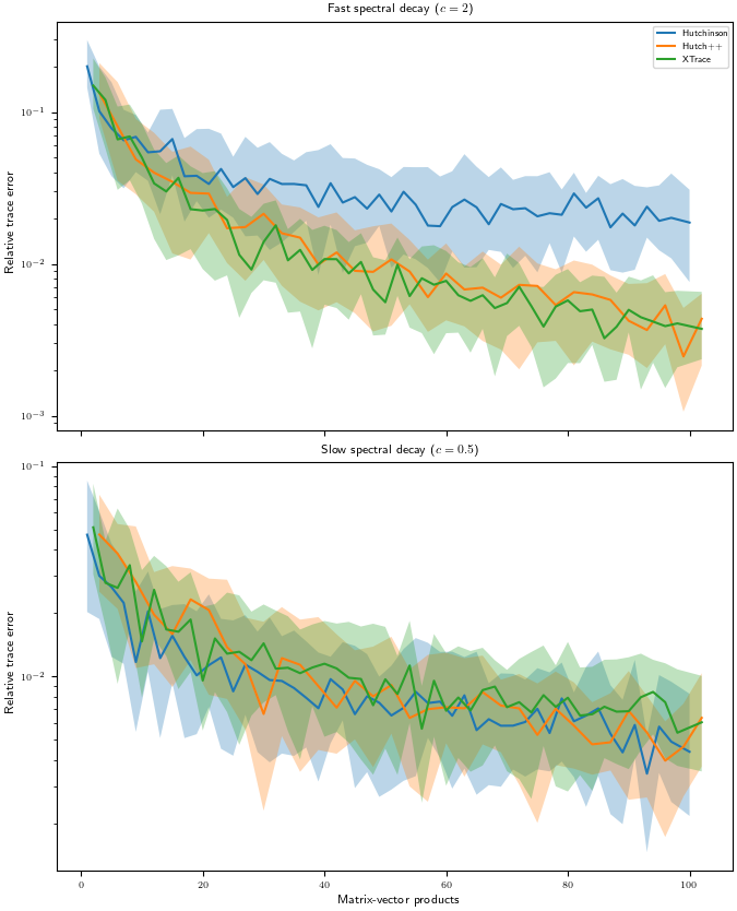
For fast spectral decay, Hutch++ and XTrace yield more accurate trace estimates than vanilla Hutchinson. For slow spectral decay, the benefits of Hutch++ and XTrace disappear. Thankfully, many curvature matrices in deep learning exhibit a decaying spectrum, which may allow Hutch++ and XTrace to improve over Hutchinson.
Diagonal estimation
Basics
Diagonal estimation is similar to trace estimation.
To give a concrete example, let’s create a power law matrix, turn it into a linear operator, and compute its diagonal for reference:
Y_mat = create_power_law_matrix()
Y = TensorLinearOperator(Y_mat)
exact_diag = Y_mat.diag()
The diagonal is a vector, which makes comparing the estimates by printing their entries tedious. Therefore, we will use the relative \(L_\infty\) error, which is the maximum entry of the absolute difference between the estimated and exact diagonal entries, divided by the maximum absolute entry of the exact diagonal.
The simplest method for diagonal estimation is Hutchinson’s method.
The idea is to estimate the diagonal from matrix-vector products with random vectors. To obtain better estimates, we can use more queries. It is common to repeat this process multiple times to get error estimates.
Let’s estimate the diagonal and see if the estimate is decent:
# matrix-vector queries for one diagonal estimate
num_matvecs = 5

# Generate estimates, repeat process multiple times so we have error bars.
estimates = [hutchinson_diag(Y, num_matvecs) for _ in range(NUM_REPEATS)]
errors = stack([relative_l_inf_error(e, exact_diag) for e in estimates])

# Calculate the median and quartiles (error bars) of the estimates
med = median(errors)
quartile1 = quantile(errors, 0.25)
quartile3 = quantile(errors, 0.75)

# Print the exact trace and the statistical measures of the estimates
print("Relative errors:")
print(f"\t- Median: {med:.3f}")
print(f"\t- First quartile (25%): {quartile1:.3f}")
print(f"\t- Third quartile (75%): {quartile3:.3f}")
Relative errors:
        - Median: 1.583
        - First quartile (25%): 1.420
        - Third quartile (75%): 1.885
Comparison
We will compare Hutchinson’s method for diagonal estimation with the XDiag method on a matrices with fast and slow spectral decay.
Here is a function that computes these relative diagonal errors for a given matrix:
NUM_MATVECS_HUTCH = linspace(1, 100, 50, dtype=int32).unique()
# XTrace requires matrix-vector products divisible by 2
NUM_MATVECS_XDIAG = (NUM_MATVECS_HUTCH + (2 - NUM_MATVECS_HUTCH % 2)).unique()


def compute_relative_diagonal_errors(Y_mat: Tensor) -> dict[str, dict[str, Tensor]]:
    """Compute the relative diagonal errors for Hutchinson's method and XDiag.

    Args:
        Y_mat: Matrix to estimate the diagonal of.

    Returns:
        Dictionary with the relative diagonal errors.
    """
    Y = TensorLinearOperator(Y_mat)
    exact_diag = Y_mat.diag()

    # compute median and quartiles for Hutchinson's method
    estimators = {
        "Hutchinson": hutchinson_diag,
        "XDiag": xdiag,
    }
    num_matvecs = [NUM_MATVECS_HUTCH, NUM_MATVECS_XDIAG]

    results = {}
    for (name, method), num_matvecs_method in zip(estimators.items(), num_matvecs):
        med = []
        quartile1 = []
        quartile3 = []

        for n in num_matvecs_method:
            estimates = [method(Y, n) for _ in range(NUM_REPEATS)]
            errors = stack([relative_l_inf_error(e, exact_diag) for e in estimates])
            med.append(median(errors))
            quartile1.append(quantile(errors, 0.25))
            quartile3.append(quantile(errors, 0.75))

        results[name] = {
            "med": as_tensor(med),
            "quartile1": as_tensor(quartile1),
            "quartile3": as_tensor(quartile3),
            "num_matvecs": num_matvecs_method,
        }

    return results
For plotting, we can re-purpose the function we used earlier to visualize the trace estimation results:
# Compute results for matrices with different spectral decay rates
Y_mat_fast = create_power_law_matrix()  # Fast spectral decay with c=2
results_fast = compute_relative_diagonal_errors(Y_mat_fast)

Y_mat_slow = create_power_law_matrix(c=0.5)  # Slow spectral decay with c=0.5
results_slow = compute_relative_diagonal_errors(Y_mat_slow)

# Plot the results for both fast and slow spectral decay
with plt.rc_context(PLOT_CONFIG):
    fig, axes = plt.subplots(nrows=2, sharex=True)
    plot_estimation_results(results_fast, axes[0], target="diagonal")
    plot_estimation_results(results_slow, axes[1], target="diagonal")
    axes[0].set_title("Fast spectral decay ($c=2$)")
    axes[1].set_title("Slow spectral decay ($c=0.5$)")

    # Remove xlabel from the first, and legend from the second, plot
    axes[0].set_xlabel(None)
    axes[1].legend().remove()

    plt.savefig("diagonal_estimation.pdf", bbox_inches="tight")
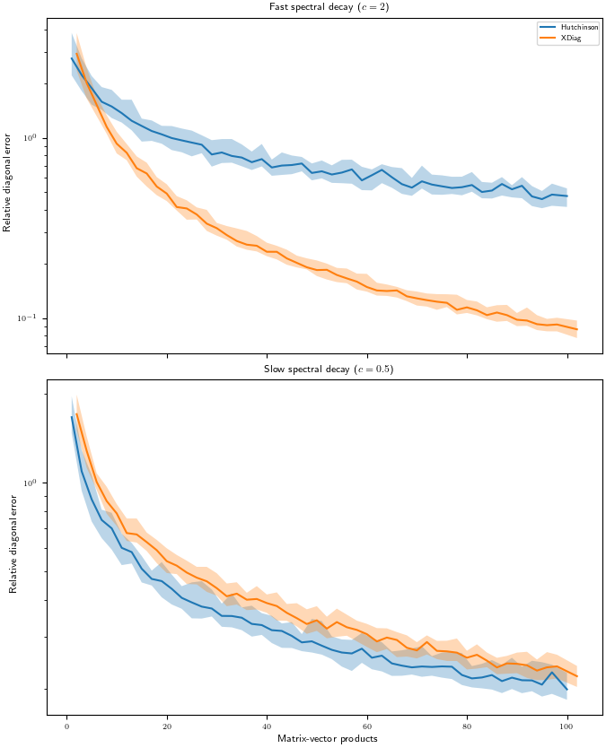
For fast spectral decay, XDiag yields more accurate diagonal estimates than vanilla Hutchinson. For slow spectral decay, its benefits disappear.
That’s all for now.
Total running time of the script: (0 minutes 58.774 seconds)